A realistic example of variational inference
Part 1: Variational Inference
In most environments, we are not able to observe all the states at play. For example, in poker, we do not see our opponent's hand, but we can observe their behavior. A statistician observing crop yields across a state cannot observe every farm for blight and disease, but the crop yields themselves can indicate the extent of any disease. Commonly, we say such situations have an observed variable $X$ and a hidden variable $Z$, where $Z$ can influence $X$, but $X$ does not influence $Z$.
| $X$ (Observed) | $Z$ (Hidden) | |
|---|---|---|
| Description | The variable we can directly measure or see | The underlying variable we cannot directly observe |
| Example 1 | Wine taste and quality ratings | Vineyard location |
| Example 2 | Crop yields across farms | Presence of blight and disease |
| Example 3 | Patient lab reports | Underlying disease state |
| Example 4 | Facial expressions and body language | Underlying emotions |
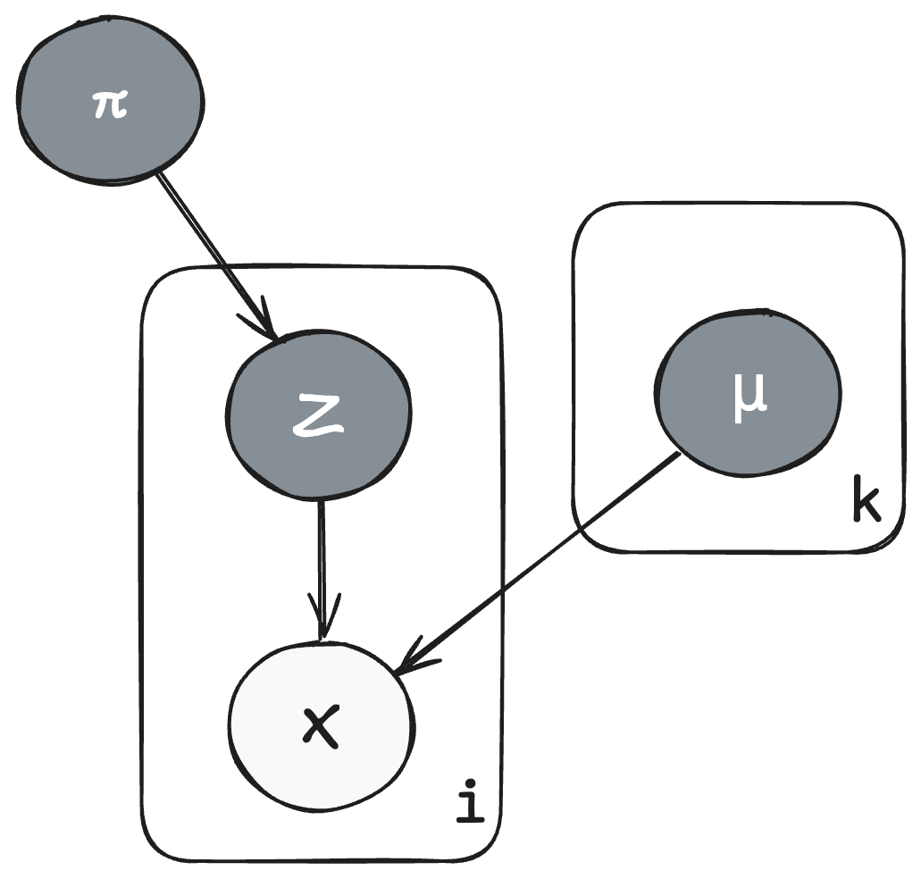
We say the variable $Z$ is the latent variable and $X$ is the observed variable.

Figure 1: Plate notation showing the relationship between latent variable $Z$ and observed variable $X$. The arrow from $Z$ to $X$ indicates that the hidden variable $Z$ influences the observed variable $X$, but not vice versa.
Usually we know the likelihood of $X$ when we know $Z$, denoted $p(x\mid z)$. For instance, it is easy to predict laboratory reports of a sick patient if we know how far their disease has progressed. With Bayes's rule, we have a pathway to compute the posterior—the disease progression given the lab report—i.e., the latent variable given the observed variable:
However, the integral in the denominator is usually intractable for most problems.
Illustration of Complexity When Computing the Denominator
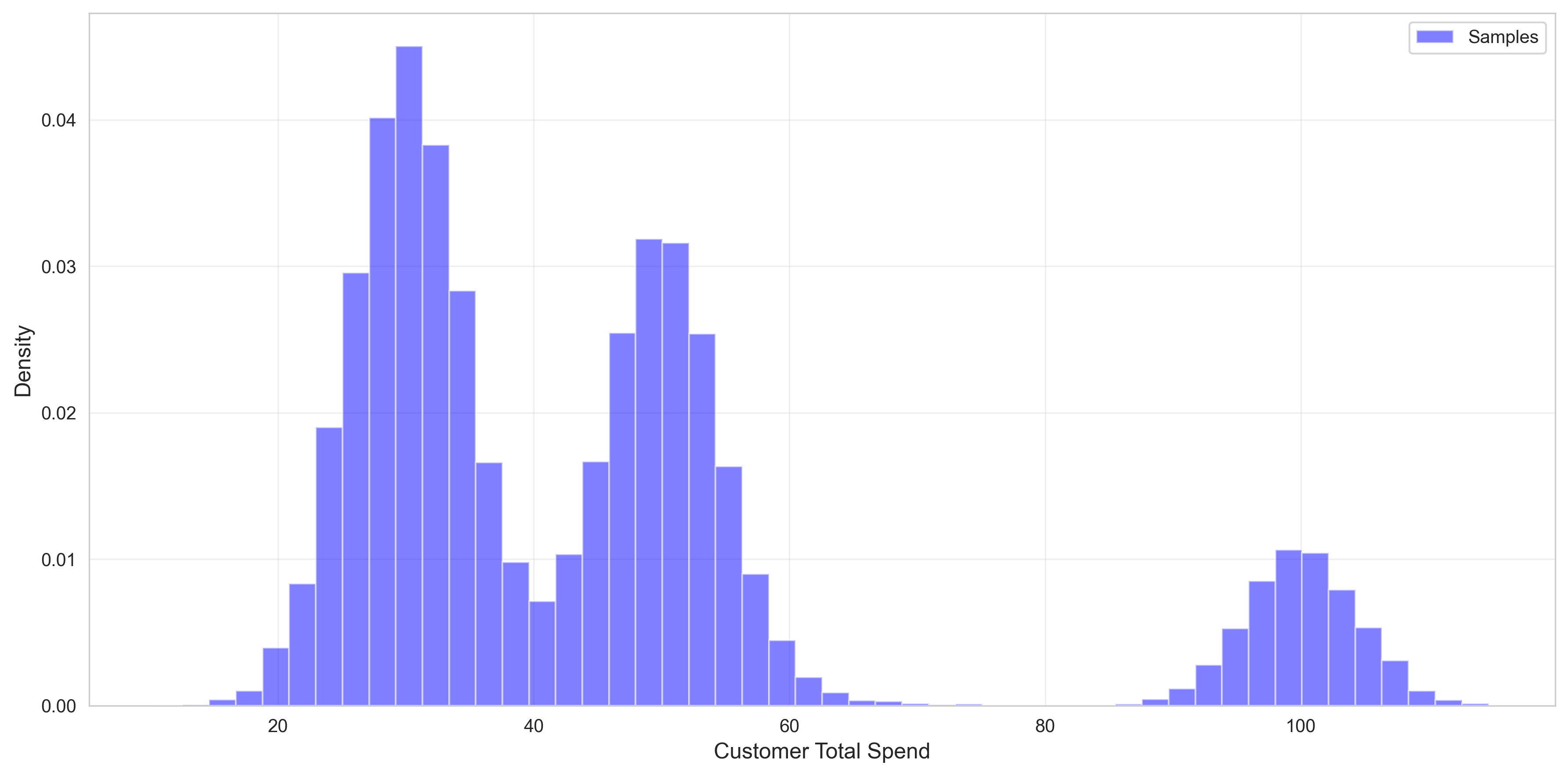
Assume you are a retail company that wants to understand consumer total spending behavior. You model your consumers as belonging to one of three categories:
- Category 1: Low spenders — $\mathcal{N}(\mu_1, \sigma^2)$
- Category 2: Medium spenders — $\mathcal{N}(\mu_2, \sigma^2)$
- Category 3: High spenders — $\mathcal{N}(\mu_3, \sigma^2)$
When the company plotted their customer lifetime spend as a histogram, the peaks on the curve matched their hypothesis.
The company can look at invoices and purchase logs to see observed total spend datapoints $\boldsymbol{x} = (x_1, \ldots, x_n)$. We don't know which category $z_i$ customer $x_i$ belongs to. We also don't know the means $\mu_k$, $k \in {1,2,3}$ for the categories, but we assume the means are normally distributed: $\color{red}{\mu_k \sim \mathcal{N}(m_0, s_0^2)}$.
We assume the probability for each category is $\color{orange}{\boldsymbol{\pi} = (\pi_1, \pi_2, \pi_3) \sim \text{Dirichlet}(\boldsymbol{\alpha})}$.
The category chosen for sample $x_i$ is $\color{purple}{z_i \sim \text{Categorical}(\boldsymbol{\pi})}$.
So, the likelihood for each spending amount $x_i$ given a specific category $z_i$ is:
The marginal for $x_i$ over all possible categories $Z_i$:
We want to find the posterior $p(\boldsymbol{z}, \boldsymbol{\pi}, \boldsymbol{\mu} \mid \boldsymbol{x})$, which is:
where the denominator $p(\boldsymbol{x})$ is the marginal likelihood, which requires integrating over all possible values of the latent variables and parameters:
This integral is intractable because we must sum over all $3^n$ possible category assignments for $\boldsymbol{z}$ and integrate over the continuous spaces of $\boldsymbol{\mu}$ and $\boldsymbol{\pi}$.
Since we do not know the exact closed form equation to infer the posterior, we approximate $p(\boldsymbol{z}, \boldsymbol{\pi}, \boldsymbol{\mu} \mid \boldsymbol{x})$ with a function family that we know.
Variational Inference on the Customer Spending Model
We don't know the posterior $p(\boldsymbol{z}, \boldsymbol{\pi}, \boldsymbol{\mu} \mid \boldsymbol{x})$, so let's define $q(\boldsymbol{z}, \boldsymbol{\pi}, \boldsymbol{\mu} \mid \boldsymbol{x})$ that we can use to approximate it. We will determine how "good" the approximation is with a divergence metric - KL divergence.
Kullback-Leibler (KL) divergence
The Kullback-Leibler (KL) divergence is a way of measuring closeness between the approximator $q$ and its target $p$
If $q$ is the same as $p$ everywhere, then $D_{KL}(q \parallel p) = 0$.
However, the issue is that we must know $p(\boldsymbol{z}, \boldsymbol{\pi}, \boldsymbol{\mu} \mid \boldsymbol{x})$ to compute this term. We can derive a more tractable objective by manipulating the KL divergence:
Rearranging:
Since KL divergence is always non-negative, we have:
The right-hand side is called the Evidence Lower Bound (ELBO):
Maximizing the ELBO with respect to $q$ is equivalent to minimizing $\text{KL}(q \parallel p)$, which makes $q$ a better approximation to the true posterior.
Choosing a variational function family
Let's choose a function for $q$, we can assume that $q(\boldsymbol{z}, \boldsymbol{\pi}, \boldsymbol{\mu}) = q(\boldsymbol{z}) q(\boldsymbol{\pi}) q(\boldsymbol{\mu})$, or that the parameters for each variable are independent of each other.
Category assignments:
where $z_i \in {1, 2, 3}$ is the category assignment for customer $i$, and $\boldsymbol{\phi}_i = (\phi_{i1}, \phi_{i2}, \phi_{i3})$ are the variational parameters defining the categorical distribution. Specifically, $\phi_{ik} = q(z_i = k)$ represents the probability that customer $i$ belongs to category $k$.
Category probabilities:
We can assume that $\pi$ has a prior from the dirichlet distribution, starting from a uniform initalization
where $\boldsymbol{\alpha}' = (1, 1, 1)$ for a uniform initialization
Category means:
Variational parameters $(m_k', s_k'^2)$ for each category $k$
The ELBO then is
The end objective is to maximize the ELBO equation above.
Implementing Stochastic Variational Inference into code
To recap, we are now solving an optimization problem where
Data: $N$ samples $x_i$ from customer spending data
Model:
Variational Parameters to Optimize:
- $\boldsymbol{\phi}_i = (\phi_{i1}, \phi_{i2}, \phi_{i3})$ for each customer $i$: The probability that customer $i$ belongs to each of the three spending categories
- $\boldsymbol{\alpha}' = (\alpha_1', \alpha_2', \alpha_3')$: Parameters of the Dirichlet distribution for category probabilities $\boldsymbol{\pi}$
- $(m_k', s_k'^2)$ for $k \in {1,2,3}$: Mean and variance parameters for the Gaussian distribution of each category mean $\mu_k$
Objective: Maximize ELBO with respect to these variational parameters
The optimization proceeds using stochastic variational inference (SVI), where we use mini-batches of data to compute noisy but unbiased estimates of the gradient. At each iteration, we:
- Sample a mini-batch of customers
- Update $\boldsymbol{\phi}$ for the mini-batch
- Scale the batch statistics by $N/\text{batch_size}$ to get unbiased estimates
- Update global parameters $\boldsymbol{\alpha}'$ and $(\boldsymbol{m}', \boldsymbol{s}'^2)$ using these scaled estimates
This stochastic approach allows us to scale to large datasets without needing to process all data points at each iteration.
Writing code for ELBO computation
As seen, the ELBO is the sum of seven terms - we will simplify them out enough to write into code and their derivatives too.
Assumption*: Here I assume readers will know that the probability mass function of the Dirichlet distribution has expectation $\mathbb{E}[\log \pi_k] = \psi(\alpha_k') - \psi(\sum_{j=1}^{3} \alpha_j')$, where $\psi$ is the digamma function. For a derivation, see this reference.
| Term | Simplification | Derivative | Notes |
|---|---|---|---|
| $\color{blue}{\sum_{i=1}^n \mathbb{E}_{z_i} \left[ \log \mathcal{N}(x_i \mid \mu_{z_i}, \sigma^2) \right]}$ | $\sum_{i=1}^n \sum_{k=1}^3 \phi_{ik} \left[ -\frac{1}{2}\log(2\pi\sigma^2) - \frac{(x_i - m_k')^2}{2\sigma^2} \right]$ | $\frac{\partial}{\partial m_k'} = \sum_{i=1}^n \phi_{ik} \frac{x_i - m_k'}{\sigma^2}$, $\frac{\partial}{\partial \phi_{ik}} = -\frac{1}{2}\log(2\pi\sigma^2) - \frac{(x_i - m_k')^2}{2\sigma^2}$ | Likelihood term - $z_i = k$, $\sigma$ is known |
| $\color{purple}{\sum_{i=1}^n \mathbb{E}_{z_i} \left[ \log \pi_{z_i} \right]}$ | $\sum_{i=1}^n \sum_{k=1}^3 \phi_{ik} \left[ \psi(\alpha_k') - \psi(\sum_{j=1}^3 \alpha_j') \right]$ | $\frac{\partial}{\partial \alpha_k'} = \sum_{i=1}^n \phi_{ik} \left[ \psi'(\alpha_k') - \psi'(\sum_j \alpha_j') \right]$, $\frac{\partial}{\partial \phi_{ik}} = \psi(\alpha_k') - \psi(\sum_{j=1}^3 \alpha_j')$ | Mixture weight term - use digamma expectation expansion |
| $\mathbb{E}_{\boldsymbol{\pi}} \left[ \color{orange}{\log \left( \frac{\Gamma(\sum_{k=1}^{3} \alpha_k)}{\prod_{k=1}^{3} \Gamma(\alpha_k)} \prod_{k=1}^{3} \pi_k^{\alpha_k - 1} \right)} \right]$ | $\log \Gamma(\sum_{k=1}^3 \alpha_k) - \sum_{k=1}^3 \log \Gamma(\alpha_k) + \sum_{k=1}^3 (\alpha_k - 1)[\psi(\alpha_k') - \psi(\sum_j \alpha_j')]$ | $\frac{\partial}{\partial \alpha_k'} = (\alpha_k - 1)[\psi'(\alpha_k') - \psi'(\sum_j \alpha_j')]$ | Prior on $\boldsymbol{\pi}$ |
| $\color{red}{\sum_{k=1}^3 \mathbb{E}_{\mu_k} \left[ \log \mathcal{N}(\mu_k \mid m_0, s_0^2) \right]}$ | $\sum_{k=1}^3 \left[ -\frac{1}{2}\log(2\pi s_0^2) - \frac{(m_k' - m_0)^2 + s_k'^2}{2s_0^2} \right]$ | $\frac{\partial}{\partial m_k'} = -\frac{m_k' - m_0}{s_0^2}$, $\frac{\partial}{\partial s_k'^2} = -\frac{1}{2s_0^2}$ | Prior on $\boldsymbol{\mu}$ - expectation taken with respect to $q(\mu_k) = \mathcal{N}(\mu_k \mid m_k', s_k'^2)$. The term $(m_k' - m_0)^2 + s_k'^2$ comes from $\mathbb{E}_q[(\mu_k - m_0)^2] = \mathbb{E}_q[\mu_k^2] - 2m_0\mathbb{E}_q[\mu_k] + m_0^2 = (s_k'^2 + m_k'^2) - 2m_0 m_k' + m_0^2 = s_k'^2 + (m_k' - m_0)^2$ |
| $\color{green}{\sum_{i=1}^n \mathbb{E}_{z_i} \left[ \log q(z_i) \right]}$ | $\sum_{i=1}^n \sum_{k=1}^3 \phi_{ik} \log \phi_{ik}$ | $\frac{\partial}{\partial \phi_{ik}} = \log \phi_{ik} + 1$ | Entropy of $q(\boldsymbol{z})$ |
| $\mathbb{E}_{\boldsymbol{\pi}} \left[ \color{teal}{\log \left( \frac{\Gamma(\sum_{k=1}^{3} \alpha_k')}{\prod_{k=1}^{3} \Gamma(\alpha_k')} \prod_{k=1}^{3} \pi_k^{\alpha_k' - 1} \right)} \right]$ | $\log \Gamma(\sum_{k=1}^3 \alpha_k') - \sum_{k=1}^3 \log \Gamma(\alpha_k') + \sum_{k=1}^3 (\alpha_k' - 1)[\psi(\alpha_k') - \psi(\sum_j \alpha_j')]$ | $\frac{\partial}{\partial \alpha_k'}$ = $\psi(\sum_j \alpha_j') - \psi(\alpha_k') + \log \phi_{ik} + \psi'(\alpha_k') - \psi'(\sum_j \alpha_j') + \psi(\alpha_k') - \psi(\sum_j \alpha_j')$ | Entropy of $q(\boldsymbol{\pi})$ |
| $\color{brown}{\sum_{k=1}^3 \mathbb{E}_{\mu_k} \left[ \log \mathcal{N}(\mu_k \mid m_k', s_k'^2) \right]}$ | $\sum_{k=1}^3 \left[ -\frac{1}{2}\log(2\pi s_k'^2) - \frac{1}{2} \right]$ | $\frac{\partial}{\partial m_k'} = 0$, $\frac{\partial}{\partial s_k'^2} = -\frac{1}{2s_k'^2}$ | Entropy of $q(\boldsymbol{\mu})$ - since $\mu_k \sim \mathcal{N}(m_k', s_k'^2)$, $\mathbb{E}_{\mu_k}[(\mu_k - m_k')^2] = s_k'^2$ |
so the code for computing the ELBO is1
2
3
4
5
6
7
8
9
10
11
12
13
14
15
16
17
18
19
20
21
22
23
24
25
26
27
28
29
30
31
32
33
34
35
36
37
38
39
40
41
42
43
44
45
46
47
48
49
50
51
52
53
54
55
56
57
58
59
60
61
62
63
64
65
66
67
68
69
70
71
72
73
74
75
76
77
78
79
80
81
82
83
84
85
86
87
88
89
90
91
92
93
94
95
96
97
98
99
100
101
102
103
104
105def compute_elbo(X, phi, alpha_variational, m_variational, s_squared_variational,
alpha_prior, m0, s0_squared, sigma_squared):
"""
Compute the Evidence Lower Bound (ELBO)
X: (n_samples, ) data points
alpha_variational: (K, ) variational parameters for π
m_variational: (K, ) variational parameters for μ
s_squared_variational: (K, ) variational parameters for σ²
alpha_prior: (K, ) prior parameters for π from Dirichlet distribution
m0: (K, ) prior parameters for μ from Normal distribution for μ
s0_squared: (K, ) prior parameters for σ² from Normal distribution for μ
sigma_squared: (K, ) known variance for σ²
"""
n = len(X)
K = len(alpha_variational)
elbo = 0.0
# E_q[log p(x | z, μ)]
# For each sample i and component k: φ_ik * log N(xi | mk', σ²)
# we multiply by phi_ik because it is equivalent of taking the expectation and stands for p(z_i = k)
for i in range(n):
for k in range(K):
log_likelihood = -0.5 * np.log(2 * np.pi * sigma_squared) - 0.5 * (X[i] - m_variational[k])**2 / sigma_squared
elbo += phi[i, k] * log_likelihood
# E_q[log p(z | π)]
# For each sample i and component k: φ_ik * E[log πk]
# E[log πk] under Dirichlet = ψ(α'k) - ψ(Σα'k)
digamma_sum = digamma(alpha_variational.sum())
for i in range(n):
for k in range(K):
expected_log_pi = digamma(alpha_variational[k]) - digamma_sum
elbo += phi[i, k] * expected_log_pi
# E_q[log p(π)] - Dirichlet prior
# log p(π) = log Dirichlet(π | α)
# E_q[log p(π)] = log Γ(Σα) - Σ log Γ(α) + Σ(α-1)E[log π]
elbo += gammaln(alpha_prior.sum()) - gammaln(alpha_prior).sum()
for k in range(K):
# E_q[log πk] where q(π) = Dirichlet(α')
# For a Dirichlet distribution q(π) = Dirichlet(α'), the expected value of log πk is:
# E_q[log πk] = ψ(α'k) - ψ(Σ_j α'j)
# where ψ is the digamma function (derivative of log Γ)
#
# This comes from the property of the Dirichlet distribution:
# If π ~ Dirichlet(α'), then E[log πk] = ψ(α'k) - ψ(Σα')
#
# Intuition: The digamma function ψ(x) ≈ log(x) for large x, so this is approximately
# log(α'k) - log(Σα'), which relates to the expected log of the normalized weight.
expected_log_pi = digamma(alpha_variational[k]) - digamma_sum
elbo += (alpha_prior[k] - 1) * expected_log_pi
# E_q[log p(μ)] - Normal prior
# For each component k: log N(μk | m0, s0²)
for k in range(K):
# E_q[log N(μk | m0, s0²)]
# The log probability of a Normal distribution is:
# log N(μk | m0, s0²) = -0.5*log(2π*s0²) - 0.5*(μk - m0)²/s0²
#
# Taking expectation with respect to q(μk) = N(mk', sk'²):
# E_q[log N(μk | m0, s0²)] = -0.5*log(2π*s0²) - 0.5*E_q[(μk - m0)²]/s0²
#
# Now we need to compute E_q[(μk - m0)²] where μk ~ N(mk', sk'²):
# E_q[(μk - m0)²] = E_q[μk² - 2μk*m0 + m0²]
# = E_q[μk²] - 2*m0*E_q[μk] + m0²
#
# For a Gaussian q(μk) = N(mk', sk'²):
# - E_q[μk] = mk' (the mean)
# - E_q[μk²] = Var(μk) + (E[μk])² = sk'² + (mk')² (second moment formula)
#
# Substituting:
# E_q[(μk - m0)²] = (sk'² + (mk')²) - 2*m0*mk' + m0²
# = sk'² + (mk')² - 2*m0*mk' + m0²
# = sk'² + (mk' - m0)²
#
# The sk'² term represents the uncertainty in our variational approximation q(μk).
# Even if mk' = m0, we still have a penalty proportional to the variance sk'².
expected_squared_diff = (m_variational[k] - m0)**2 + s_squared_variational[k]
log_prior = -0.5 * np.log(2 * np.pi * s0_squared) - 0.5 * expected_squared_diff / s0_squared
elbo += log_prior
# -E_q[log q(z)]
# Entropy of categorical: -Σi Σk φ_ik log φ_ik
for i in range(n):
for k in range(K):
if phi[i, k] > 1e-10: # Avoid log(0)
elbo -= phi[i, k] * np.log(phi[i, k])
# -E_q[log q(π)]
# Entropy of Dirichlet
elbo -= gammaln(alpha_variational.sum()) - gammaln(alpha_variational).sum()
for k in range(K):
expected_log_pi = digamma(alpha_variational[k]) - digamma_sum
elbo -= (alpha_variational[k] - 1) * expected_log_pi
# -E_q[log q(μ)]
# Entropy of Gaussians: 0.5*log(2πe*s²)
for k in range(K):
entropy = 0.5 * np.log(2 * np.pi * np.e * s_squared_variational[k])
elbo += entropy
return elbo
Similarly we can write code for updating the variational parameters phi, alpha and m_k, s_k and do gradient ascent to update $q$'s parameters, as shown in the animation below.